Scale-Invariant Feature Transform
Contents
Introduction
Recognizing objects in images is one of the most important problems in computer vision. A common approach is to first extract the feature descriptions of the objects to be recognized from reference images, and store such descriptions in a database. When there is a new image, its feature descriptions are extracted and compared to the object descriptions in the database to see if the image contains any object we are looking for. In real-life applications, the objects in the images to be processed can differ from the reference images in many way:
- Scale, i.e. size of the object in the image
- Orientation
- Viewpoint
- Illumination
- Partially covered
The Algorithm
The SIFT algorithm contains several steps, illsutrated in the processing pipeline of SIFT below.
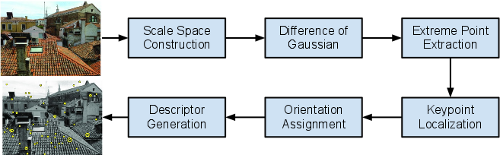
In this assignment, we exclude the last step descriptor generation as it is only a post processing of the keypoint information.
Scale Space Construction
In SIFT, an image pyramid is built as the first step: the image is process with multiple Gaussian filters. The output of each filter is called a scale. Then the algorithm moves on to the next octave by down-scale the image by a factor of 2, and produce another S Gaussian blurred images. This process continues until the image size reach certain limit. The scale space contributes to the scale invariance of SIFT. An example of the scale space is illustrated below.
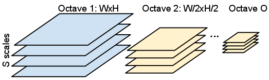
In the reference implementation, the scale space construction is separated into two steps. The first step is to build the octave bases. An image is downsampled into multiple octaves, each has half of the width and height of the octave at a lower level. An image is downsampled multiple times to create as many octaves as possible, but the top two octaves are discarded due to their small size. The number of octaves O = log2(min(width, height)) - 2. The second step is build the scale space from octave bases. Each octave is smoothed with multiple Gaussian filters of different sigma values to create multiple scales of the image. In the reference implementation, the scale-per-octave value S = 6, which means each octave will be smoothed by 6 different Gaussian kernels to create 6 different scales of the image.
Difference-of-Gaussian
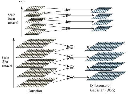
The Difference-of-Gaussian (DoG) images are taken from adjacent Gaussian-blurred images per octave. The follow figure illustrate the idea of scale space construction and DoG calculation. For each octave, images of adjacent scales will subtract each other to create Difference of Gaussian (DoG) images. There will be Ox(S-1) number of DoG images in total.
Extreme Points Extraction
keypoints are identified as local minima/maxima of the DoG images across scales. This is done by comparing each pixel in the DoG images to its eight neighbors at the same scale and nine corresponding neighboring pixels in each of the neighboring scales. If the pixel value is the maximum or minimum among all compared pixels, it is selected as a candidate keypoint.
Keypoint Localization
Extreme points extraction usually produces too many keypoint candidates. The following two kinds of candidates are eliminated:
- Low-contrast keypoints
- Edge responses
Orientation Assignment
The orientation assignment stage calculates orientation of each keypoint base on gradient. The magnitude and direction calculations for the gradient are done for every pixel in a neighboring window around the keypoint in the Gaussian-blurred image. Each pixel votes in a orientation histogram. In the provided reference implementation, the algorithm only picks the maximum orientation in the histogram as the orientation of a keypoint. More advanced implementations, e.g. sift++, lowe's sift, etc., consider all dominant orientations (>80% peak) as the orientations of a keypoint. In all these implementations, the orientation assignment is to ensure the keypoints are invariant to rotation.
Reference Implementation
A reference implementation of the SIFT algorithm in C is available. You can download this zip file.
SIFT related source files are in src/. Codes not directly related to SIFT are located in util/. You should focus on the codes in src/. The reference program produces two outputs that can be used for verification:
- A ppm image contains the input and keypoints detected
- A text file skey that specify the position (x, y), the scale and orientation of each keypoint
Only a small image box.pgm is in the zip file. You can use it to test your program. A set of larger images are available here.
Remarks
- The timer utility functions in util/timer.* can be used to measure the execution time. The usage is shown in sift() in src/sift.c
- A match.c is available to match the results generated by the reference code and your modified code.
Feel free to contact us if you find any problem in the reference code.
Useful Links